
For SEO experts, basic Google updates are a way of life. It will happen at least once – if not several times – a year.
Naturally, there will be winners and losers.
So while Google doesn’t disclose most of the ranking factors behind its algorithm updates, there are things we can do to get a greater understanding of what’s going on, in terms of:
- Website content that is affected.
- Sites operating in your search space.
- Results types.
The limit is your imagination, your questions (based on your SEO knowledge), and of course, your data.
This code will cover aggregations at the search engine results page (SERP) level (Crosssite Category Comparison), and the same principles can be applied to other views of core update as result types (thinking snippets and other views mentioned above).
Using Python to compare SERPs
The general principle is to compare the SERPs before and after the core update, which will give us some clue as to what’s going on.
We’ll start by importing our Python libraries:
import re
import time
import random
import pandas as pd
import numpy as np
import datetime
from datetime import timedelta
from plotnine import *
import matplotlib.pyplot as plt
from pandas.api.types import is_string_dtype
from pandas.api.types import is_numeric_dtype
import uritools
pd.set_option('display.max_colwidth', None)
%matplotlib inline
In identifying a few variants, we will focus on ON24.com as they lost their primary update.
root_domain = 'on24.com'
hostdomain = 'www.on24.com'
hostname="on24"
full_domain = 'https://www.on24.com'
site_name="ON24"
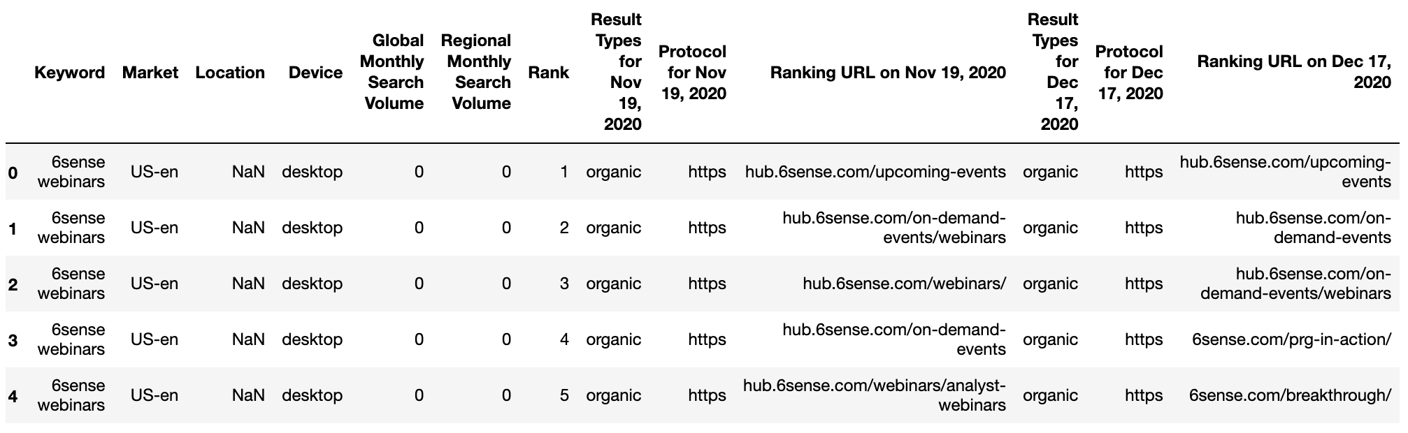
When reading the data, we use an export from GetSTAT which contains a useful report that allows you to compare the SERPs of your keywords before and after.
This SERPs report is available from other rank tracking providers such as Search engine optimization monitoring And the Advanced web ranking – No preferences or approvals on my part!
getstat_ba_urls = pd.read_csv('data/webinars_top_20.csv', encoding = 'UTF-16', sep = 't')
getstat_raw.head()
getstat_ba_urls = getstat_raw
Create URLs by joining the protocol and the URL string to get the full URL of the pre- and post-update collation.
getstat_ba_urls['before_url'] = getstat_ba_urls['Protocol for Nov 19, 2020'] + '://' + getstat_ba_urls['Ranking URL on Nov 19, 2020']
getstat_ba_urls['after_url'] = getstat_ba_urls['Protocol for Dec 17, 2020'] + '://' + getstat_ba_urls['Ranking URL on Dec 17, 2020']
getstat_ba_urls['before_url'] = np.where(getstat_ba_urls['before_url'].isnull(), '', getstat_ba_urls['before_url'])
getstat_ba_urls['after_url'] = np.where(getstat_ba_urls['after_url'].isnull(), '', getstat_ba_urls['after_url'])
To get the ranges of the URLs to rank, we create a copy of the URL in a new column, and remove the subdomains using the if statement included in the list comprehension:
getstat_ba_urls['before_site'] = [uritools.urisplit(x).authority if uritools.isuri(x) else x for x in getstat_ba_urls['before_url']]
stop_sites = ['hub.', 'blog.', 'www.', 'impact.', 'harvard.', 'its.', 'is.', 'support.']
getstat_ba_urls['before_site'] = getstat_ba_urls['before_site'].str.replace('|'.join(stop_sites), '')
The comprehension list is iterated to extract domains after the update.
getstat_ba_urls['after_site'] = [uritools.urisplit(x).authority if uritools.isuri(x) else x for x in getstat_ba_urls['after_url']]
getstat_ba_urls['after_site'] = getstat_ba_urls['after_site'].str.replace('|'.join(stop_sites), '')
getstat_ba_urls.columns = [x.lower() for x in getstat_ba_urls.columns]
getstat_ba_urls = getstat_ba_urls.rename(columns = {'global monthly search volume': 'search_volume'
                                                   })
getstat_ba_urls
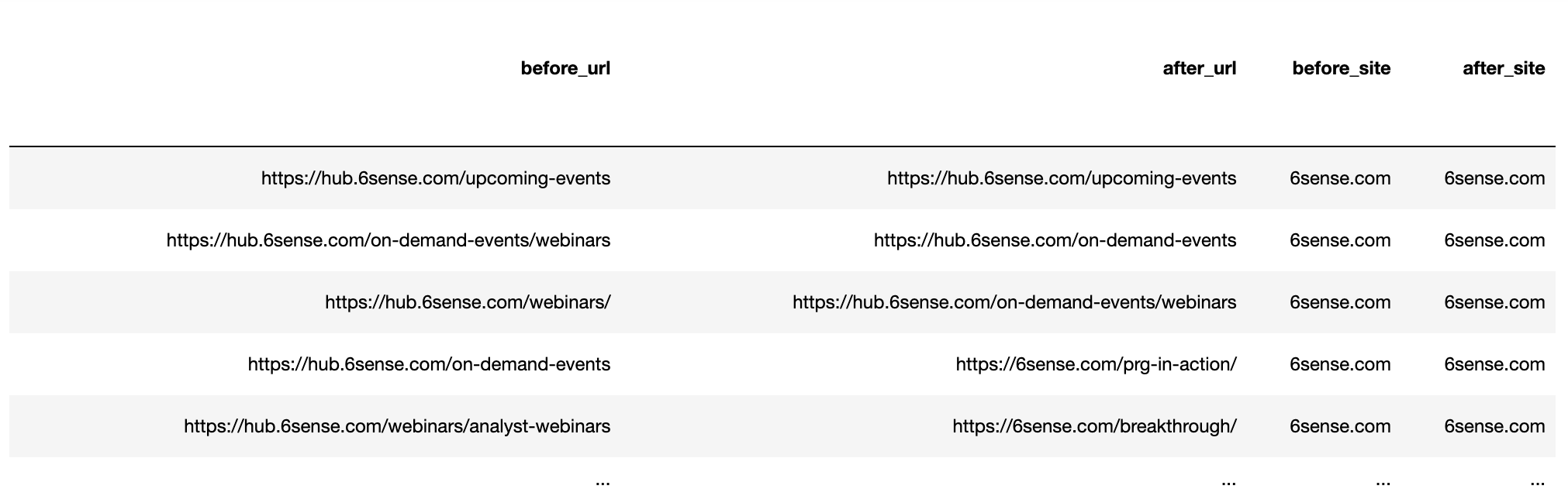 Screenshot by the author, January 2022
Eliminate multiple URLs
The next step is to remove multiple URLs to rank by the same domain for each SERP keyword. We will divide the data into two groups, before and after.
Then we will group by keyword and cancel the iterator:
getstat_bef_unique = getstat_ba_urls[['keyword', 'market', 'location', 'device', 'search_volume', 'rank',
       'result types for nov 19, 2020', 'protocol for nov 19, 2020',
       'ranking url on nov 19, 2020', 'before_url', 'before_site']]
getstat_bef_unique = getstat_bef_unique.sort_values('rank').groupby(['before_site', 'device', 'keyword']).first()
getstat_bef_unique = getstat_bef_unique.reset_index()
getstat_bef_unique = getstat_bef_unique[getstat_bef_unique['before_site'] != '']
getstat_bef_unique = getstat_bef_unique.sort_values(['keyword', 'device', 'rank'])
getstat_bef_unique = getstat_bef_unique.rename(columns = {'rank': 'before_rank',
                                                          'result types for nov 19, 2020': 'before_snippets'})
getstat_bef_unique = getstat_bef_unique[['keyword', 'market', 'device', 'before_snippets', 'search_volume',
                                         'before_url', 'before_site', 'before_rank'
                                        ]]
getstat_bef_unique
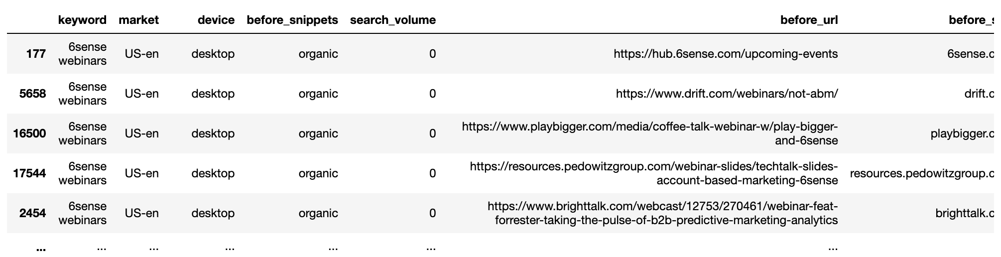 Screenshot by the author, January 2022
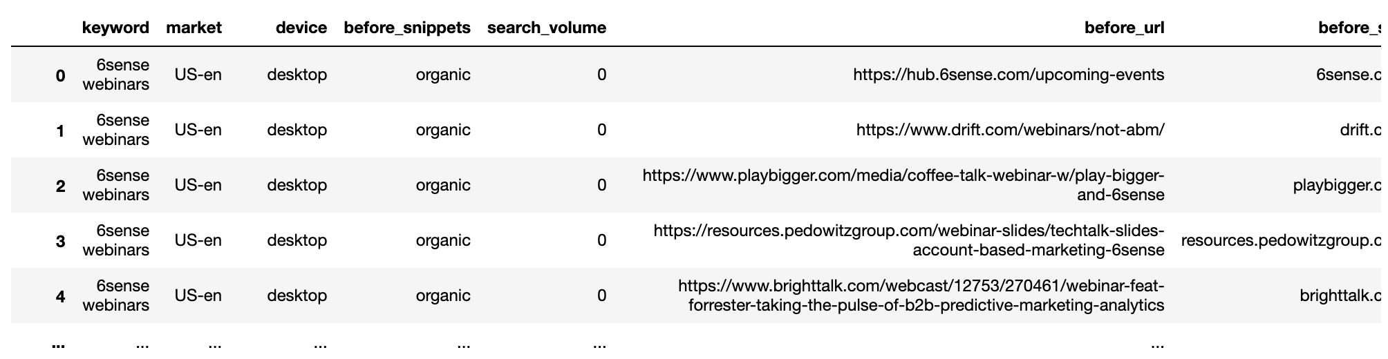
The procedure is repeated for the subsequent data set.
getstat_aft_unique = getstat_ba_urls[['keyword', 'market', 'location', 'device', 'search_volume', 'rank',
       'result types for dec 17, 2020', 'protocol for dec 17, 2020',
       'ranking url on dec 17, 2020', 'after_url', 'after_site']]
getstat_aft_unique = getstat_aft_unique.sort_values('rank').groupby(['after_site', 'device', 'keyword']).first()
getstat_aft_unique = getstat_aft_unique.reset_index()
getstat_aft_unique = getstat_aft_unique[getstat_aft_unique['after_site'] != '']
getstat_aft_unique = getstat_aft_unique.sort_values(['keyword', 'device', 'rank'])
getstat_aft_unique = getstat_aft_unique.rename(columns = {'rank': 'after_rank',
                                                          'result types for dec 17, 2020': 'after_snippets'})
getstat_aft_unique = getstat_aft_unique[['keyword', 'market', 'device', 'after_snippets', 'search_volume',
                                         'after_url', 'after_site', 'after_rank'
                                        ]]
Segmentation of SERP sites
When it comes to core updates, most of the answers tend to be in the SERPs. This is where we can see which sites are being rewarded and which others are losing.
With the datasets excluded and separated, we will work on finding the common competitors so we can begin to manually segment them which will help us visualize the impact of the update.
serps_before = getstat_bef_unique
serps_after = getstat_aft_unique
serps_before_after = serps_before_after.merge(serps_after, left_on = ['keyword', 'before_site', 'device', 'market', 'search_volume'],
                                                right_on = ['keyword', 'after_site', 'device', 'market', 'search_volume'], how = 'left')
Clean up order columns from nulls (NAN Not a Number) using the np.where() function which is the Panda equivalent of Excel if formula.
serps_before_after['before_rank'] = np.where(serps_before_after['before_rank'].isnull(), 100, serps_before_after['before_rank'])
serps_before_after['after_rank'] = np.where(serps_before_after['after_rank'].isnull(), 100, serps_before_after['after_rank'])
Some metrics calculated to show the rank difference before vs after, and whether the URL has changed.
serps_before_after['rank_diff'] = serps_before_after['before_rank'] - serps_before_after['after_rank']
serps_before_after['url_change'] = np.where(serps_before_after['before_url'] == serps_before_after['after_url'], 0, 1)
serps_before_after['project'] = site_name
serps_before_after['reach'] = 1
serps_before_after
 Screenshot by the author, January 2022
Collect the winning spots
With the data cleaned up, we can now group to see which sites are most dominant.
To do this, we define a function that computes a weighted average ranking by search volume.
Not all keywords matter which helps make the analysis more meaningful if you pay attention to which keywords get the most searches.
def wavg_rank(x):
    names = {'wavg_rank': (x['before_rank'] * (x['search_volume'] + 0.1)).sum()/(x['search_volume'] + 0.1).sum()}
    return pd.Series(names, index=['wavg_rank']).round(1)

rank_df = serps_before_after.groupby('before_site').apply(wavg_rank).reset_index()
reach_df = serps_before_after.groupby('before_site').agg({'reach': 'sum'}).sort_values('reach', ascending = False).reset_index()

commonstats_full_df = rank_df.merge(reach_df, on = 'before_site', how = 'left').sort_values('reach', ascending = False)
commonstats_df = commonstats_full_df.sort_values('reach', ascending = False).reset_index()
commonstats_df.head()
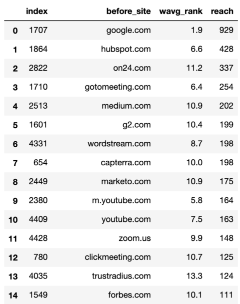 Screenshot by the author, January 2022
While the weighted average rank is important, reach is also important as it tells us the breadth of a site’s presence in Google i.e. the number of keywords.
Reach also helps us prioritize the sites we want to include in our segmentation.
Partitioning works with the np.select function which is similar to Excel’s huge nested if formula.
First, we list our terms.
domain_conds = [
    commonstats_df['before_site'].isin(['google.com', 'medium.com', 'forbes.com', 'en.m.wikipedia.org',
                                        'hbr.org', 'en.wikipedia.org', 'smartinsights.com', 'mckinsey.com',
                                        'techradar.com','searchenginejournal.com',
                                        'cmswire.com']),
    commonstats_df['before_site'].isin(['on24.com', 'gotomeeting.com', 'marketo.com', 'zoom.us', 'livestorm.co',
                                        'hubspot.com', 'drift.com', 'salesforce.com', 'clickmeeting.com',
                                        'qualtrics.com', 'workcast.com', 'livewebinar.com', 'getresponse.com',
                                        'superoffice.com', 'myownconference.com', 'info.workcast.com']),
    commonstats_df['before_site'].isin([ 'neilpatel.com', 'ventureharbour.com', 'wordstream.com',
                                        'business.tutsplus.com', 'convinceandconvert.com']),
    commonstats_df['before_site'].isin(['trustradius.com', 'g2.com', 'capterra.com', 'softwareadvice.com',
                                        'learn.g2.com']),
    commonstats_df['before_site'].isin(['youtube.com', 'm.youtube.com', 'facebook.com', 'linkedin.com',
                                        'business.linkedin.com',
                                       ])
]
Then we create a list of values that we want to set for each condition.
segment_values = ['publisher', 'martech', 'consulting', 'reviews', 'social_media']
Then create a new column and use np.select to assign values to it using our lists as arguments.
commonstats_df['segment'] = np.select(domain_conds, segment_values, default="other")
commonstats_df = commonstats_df[['before_site', 'segment', 'reach', 'wavg_rank']]
commonstats_df
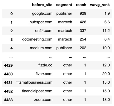 Screenshot by the author, January 2022
Domains are now fragmented which means we can start the fun collecting to see what kinds of sites have benefited from the update and degraded.
# SERPs Before and After Rank
serps_stats = commonstats_df[['before_site', 'segment']]
serps_segments = commonstats_df.segment.to_list()
We join the unique data before the SERPs with the SERP segments table created directly above to split the rank URLs using the merge function.
A merge function that uses the “eft” parameter is equivalent to Excel’s vlookup or index matching function.
serps_before_segmented = getstat_bef_unique.merge(serps_stats, on = 'before_site', how = 'left')
serps_before_segmented = serps_before_segmented[~serps_before_segmented.segment.isnull()]
serps_before_segmented = serps_before_segmented[['keyword', 'segment', 'device', 'search_volume', 'before_snippets',
                             'before_rank', 'before_url', 'before_site']]
serps_before_segmented['count'] = 1
serps_queries = serps_before_segmented['keyword'].to_list()
serps_queries = list(set(serps_queries))
serps_before_segmented
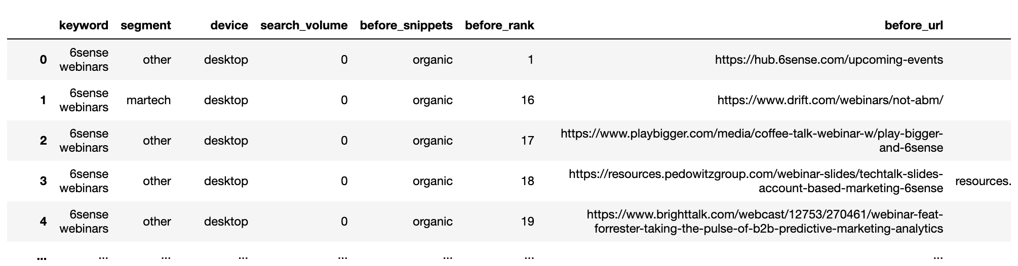 Screenshot by the author, January 2022
Compilation before SERPs:
def wavg_rank_before(x):
    names = {'wavg_rank_before': (x['before_rank'] * x['search_volume']).sum()/(x['search_volume']).sum()}
    return pd.Series(names, index=['wavg_rank_before']).round(1)

serps_before_agg = serps_before_segmented
serps_before_wavg = serps_before_agg.groupby(['segment', 'device']).apply(wavg_rank_before).reset_index()
serps_before_sum = serps_before_agg.groupby(['segment', 'device']).agg({'count': 'sum'}).reset_index()
serps_before_stats = serps_before_wavg.merge(serps_before_sum, on = ['segment', 'device'], how = 'left')
serps_before_stats = serps_before_stats.rename(columns = {'count': 'before_n'})
serps_before_stats
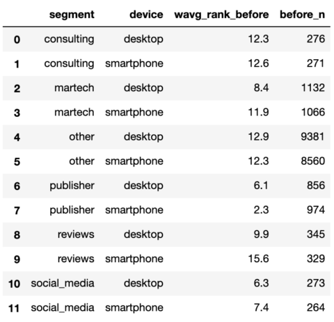 Screenshot by the author, January 2022
Repeat the procedure after the SERPs.
# SERPs  After Rank
aft_serps_segments = commonstats_df[['before_site', 'segment']]
aft_serps_segments = aft_serps_segments.rename(columns = {'before_site': 'after_site'})
serps_after_segmented = getstat_aft_unique.merge(aft_serps_segments, on = 'after_site', how = 'left')
serps_after_segmented = serps_after_segmented[~serps_after_segmented.segment.isnull()]
serps_after_segmented = serps_after_segmented[['keyword', 'segment', 'device', 'search_volume', 'after_snippets',
                             'after_rank', 'after_url', 'after_site']]
serps_after_segmented['count'] = 1
serps_queries = serps_after_segmented['keyword'].to_list()
serps_queries = list(set(serps_queries))
def wavg_rank_after(x):
    names = {'wavg_rank_after': (x['after_rank'] * x['search_volume']).sum()/(x['search_volume']).sum()}
    return pd.Series(names, index=['wavg_rank_after']).round(1)
serps_after_agg = serps_after_segmented
serps_after_wavg = serps_after_agg.groupby(['segment', 'device']).apply(wavg_rank_after).reset_index()
serps_after_sum = serps_after_agg.groupby(['segment', 'device']).agg({'count': 'sum'}).reset_index()
serps_after_stats = serps_after_wavg.merge(serps_after_sum, on = ['segment', 'device'], how = 'left')
serps_after_stats = serps_after_stats.rename(columns = {'count': 'after_n'})
serps_after_stats
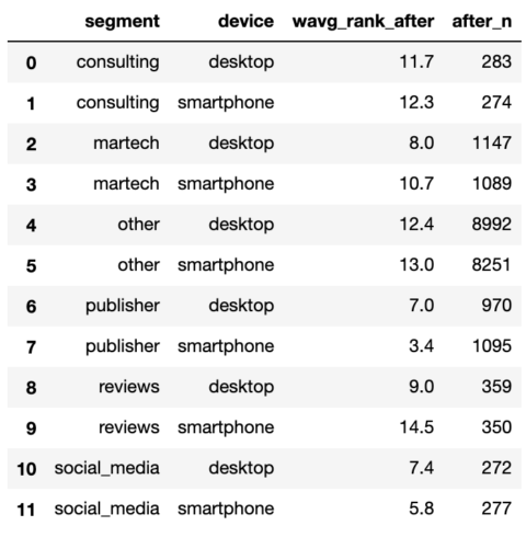 Screenshot by the author, January 2022
With both SERPs summed up, we can join them and start making comparisons.
serps_compare_stats = serps_before_stats.merge(serps_after_stats, on = ['device', 'segment'], how = 'left')
serps_compare_stats['wavg_rank_delta'] = serps_compare_stats['wavg_rank_after'] - serps_compare_stats['wavg_rank_before']
serps_compare_stats['sites_delta'] = serps_compare_stats['after_n'] - serps_compare_stats['before_n']
serps_compare_stats
 Screenshot by the author, January 2022
Although we can see that publisher sites seem to gain the most thanks to more keywords they rank for, an image will definitely tell the 1,000 more words in your PowerPoint suite.
We will endeavor to do this by resampling the data into a long format favored by the Python ‘plotnine’ graphics package.
serps_compare_viz = serps_compare_stats
serps_rank_viz = serps_compare_viz[['device', 'segment', 'wavg_rank_before', 'wavg_rank_after']].reset_index()
serps_rank_viz = serps_rank_viz.rename(columns = {'wavg_rank_before': 'before', 'wavg_rank_after': 'after', })
serps_rank_viz = pd.melt(serps_rank_viz, id_vars=['device', 'segment'], value_vars=['before', 'after'],
                     var_name="phase", value_name="rank")
serps_rank_viz
serps_ba_plt = (
    ggplot(serps_rank_viz, aes(x = 'segment', y = 'rank', colour="phase",
                             fill="phase")) +
    geom_bar(stat="identity", alpha = 0.8, position = 'dodge') +
    labs(y = 'Google Rank', x = 'phase') +
    scale_y_reverse() +
    theme(legend_position = 'right', axis_text_x=element_text(rotation=90, hjust=1)) +
    facet_wrap('device')
)
serps_ba_plt
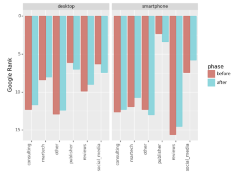 Screenshot by the author, January 2022
And we have our first visualization, which shows us how most types of sites have gained in ranking which is only half the story.
Let’s also look at the number of entries in the top 20.
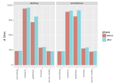 Screenshot by the author, January 2022
Ignoring the “Other” slide, we can see that Martech and publishers were the main winners by expanding the reach of their keywords.
summary
It only took a bit of code to create one schema with all the cleanup and grouping.
However, principles can be applied to achieve extended winner-and-loser perspectives such as:
- domain level.
- Internal website content.
- Results types.
- The results of cannibalism.
- Classification of URL content types (blogs, offer pages, etc.).
Most SERP reports will contain the data needed to perform the expanded bids listed above.
While it may not explicitly reveal the main ranking factor, the views can tell you a lot about what’s going on, help you explain the base update to your peers, and generate hypotheses to test whether you’re one of the less fortunate looking to recover.
More resources:
- Introduction to Python and machine learning for technical SEO
- Python SEO: Top keyword opportunities within an amazing distance
- Advanced Technical SEO: A Complete Guide
Featured image: Pixel Hunter/Shutterstock